For a physics student, the Legendre transform is one of those mathematical techniques which textbooks often don’t give as much love and attention as compared to the Fourier or Laplace transforms. Yet, it’s used in key pieces of classical physics: you may have encountered it in thermodynamics, where it is used to relate the internal energy of a system to other thermodynamic potentials like the free energy or enthalpy. Or maybe you came across the Legendre transform in classical mechanics as the link between the Lagrangian and the Hamiltonian.

I found the Legendre transform to be opaque and less intuitive than other operations:

• I did not understand why the Legendre transform \(G(p)\) of a function \(F(x)\) is defined by \(G = p\,x - F\).

• Why is \(p\) the derivative of \(F\)? How is it an independent variable?

• What is the intuition behind the Legendre transform anyway?

If you’ve asked the same questions, then my goal with this post is to share a clear exposition of what the Legendre transform is, as well as why it is the right way to describe the deep connection between energy, temperature and entropy.

Curves and tangent lines

I’ll start by posing a seemingly unrelated problem, but it contains all the intuition you’ll need to understand Legendre transforms:

If I give you a curve in the \(x\)-\(y\) plane, how would you describe its tangent lines?

Here is a concrete example: say the curve is the parabola \(F(x) = x^2\). Pick a point on the parabola, say \((1, 1)\), and draw the tangent line:

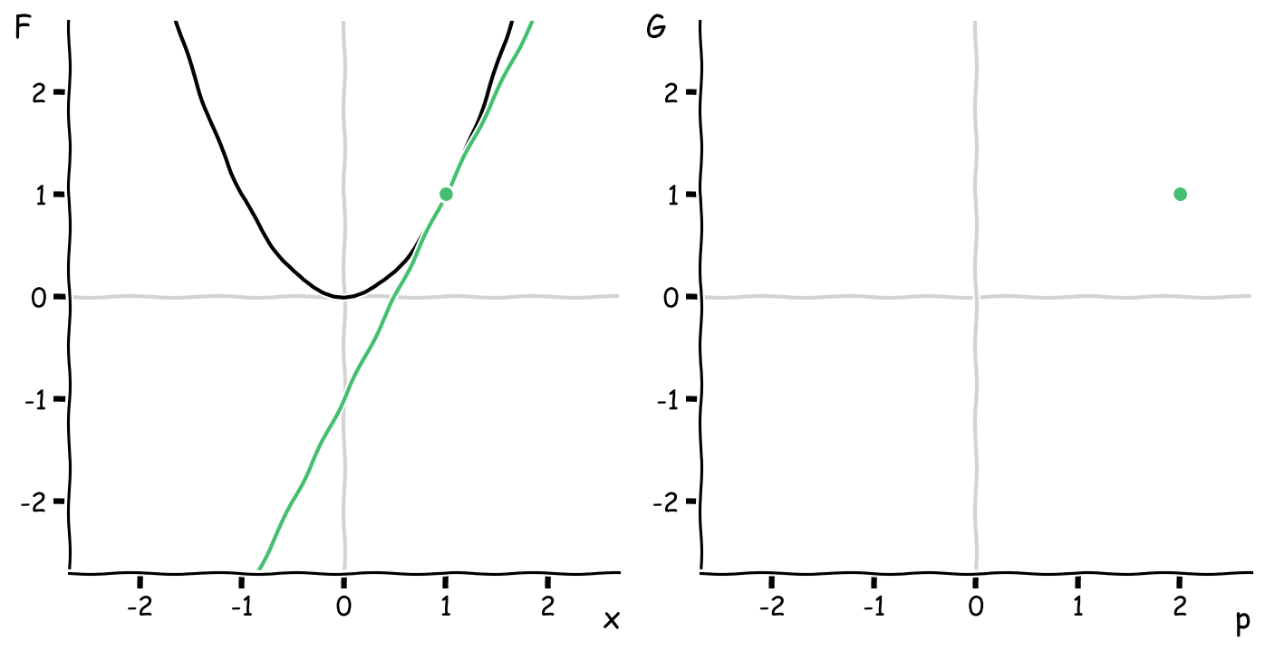
One way to describe this particular tangent line is by its slope and \(y\)-intercept, which are \(2\) and \(-1\) respectively. It’s formula is

\[y = 2x - 1\]

Take another point on the parabola, say \((\frac{1}{2}, \frac{1}{4})\) and again draw the tangent line. Its slope is \(1\), and the \(y\)-intercept is \(-\frac{1}{4}\), so the formula for this second tangent line is

\[y = x - \frac{1}{4}\]

Imagine repeating this process for a bunch of points on the curve and tabulating the slopes, which I’ll call \(p\), and for reasons I’ll explain further down, the negative of the \(y\)-intercepts \(G\). The result is a table like this:

\(x\)	\(F\)	\(p\)	\(G\)
-1	1	-2	1
-1/2	1/4	-1	1/4
0	0	0	0
1/2	1/4	1	1/4
1	1	2	1

Just as we have plotted \(F\) against \(x\), we can construct a new function \(G(p)\) by plotting the intercepts \(G\) against the slopes \(p\):

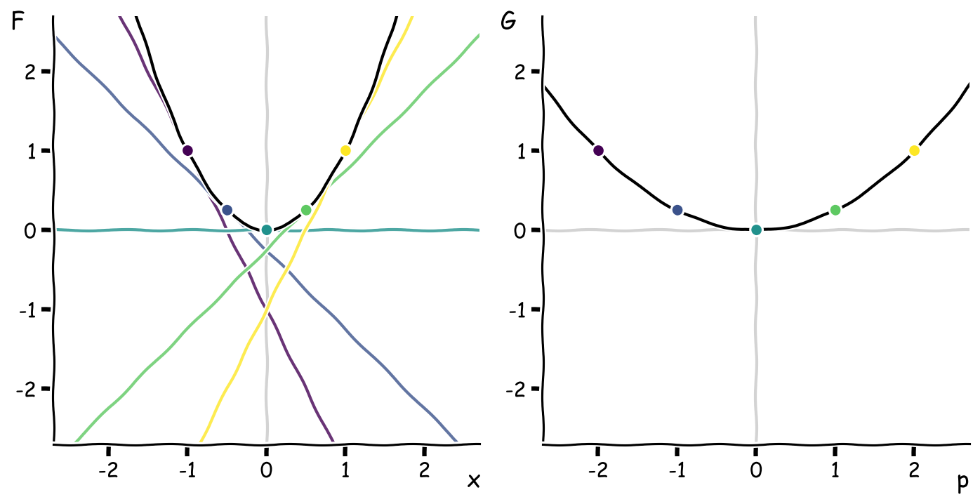
This new curve of the intercepts vs. slopes is the Legendre transform. That’s it!

The Legendre transform of a function is the negative \(y\)-intercepts of its tangent lines plotted against their slopes.

A neat property of the Legendre transform is that it contains all the information of the original function, but encoded in terms of different variables \(p\) and \(G\). In fact, the curve we constructed is an example of a dual curve, which is an idea from the field of projective geometry: plane curves can be described equally well as a set of points or as a set of corresponding tangent lines.

Now you can answer the original question posed:

If I give you a curve in the \(x\)-\(y\) plane, how would you describe its tangent lines?

Use the Legendre transform!

In the above example, the function \(G(p)\) looks suspiciously like a parabola as well. How would you compute the Legendre transform algebraically?

From curves to equations

Let’s rephrase the question in mathematical notation: given a function \(F(x)\) with independent variable \(x\), what is the procedure to compute the Legendre transform \(G(p)\), where the independent variable \(p\) ranges over the slopes of the tangent lines?

The trick is to consider the right triangle formed by the points on the function \(F\) and the negative \(y\)-intercept \(G\):

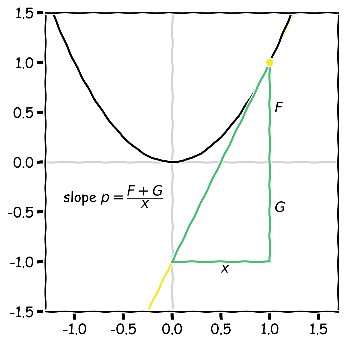
Adding up the length of the two vertical line segments, the height of the triangle is \(F+G\). The width is \(x\). The slope \(p\) of the triangle is

\[p = \frac{F + G}{x}\]

which when rearranged gives a beautifully symmetric formula:

\[F + G = p x\]

You’ll notice that if you swap \(F \leftrightarrow G\) and \(x \leftrightarrow p\), the formula remains unchanged. This means that if you apply the Legendre transform twice, you’ll get back the original function: the transform is its own inverse, an involution.

Now you see the reason we worked with negative \(y\)-intercept: if we had used the regular \(y\)-intercept, the triangle height would have been \(F - G\), and the Legendre transform so defined would have an extra minus sign floating around and not be an involution.

Aside: not everyone defines the Legendre transform this way, so pay attention to minus sign conventions in the literature.

One other property to note is that if they were phyiscal quantities, the Legendre transform \(G\) must have the same units as \(F\). For example, if \(F\) had units of energy, then \(G\) must also be a measure of energy. Likewise, the product \(p x\) must also have units of energy. [How does this relate to \(p\) and \(x\) being conjugate variables? What’s the definition of a conjugate variable and what physical process do they represent?]

Finally, solving for \(G\), we get

\[G = p\, x - F\]

While this formula makes sense in terms of segment lengths of the triangle, what is lost is the notion of what is the independent variable. Since the Legendre transform is a function of the tangent line slopes, what we do is the following: given the input \(F(x)\)

1. Find the tangent line slopes by taking the derivative \(p = f(x) \equiv F'(x)\)
2. Invert this equation to get \(x = f^{-1}(p)\).
3. Insert into the expression \(p x - F(x)\) to eliminate \(x\) in favor of \(p\)

In summary, this is the prescription for finding the Legendre transform:

\[\boxed{ \begin{gather} G(p) = p \, f^{-1}(p) - F(f^{-1}(p)) \\ \text{where } f = F' \text{ and } f^{-1} \text{ is obtained by inverting } p = f(x) \end{gather} }\]

Now we can answer the question of whether the Legendre transform of \(F(x) = x^2\) is also a parabola:

1. The derivative is \(p = f(x) = 2x\)
2. The original coordinate in terms of the derivative is \(x = f^{-1}(p) = p / 2\)
3. The Legendre transform is \(G(p) = p \cdot p/2 - (p/2)^2 = p^2 / 4\)

Yes, it’s a parabola! Also, you can check that applying the transform again to \(G(p) = p^2/4\) will recover the original function, showing that the transform is an involution.

Aside on notation: I will use lowercase letters \(f = F'\) and \(g = G'\) to denote the derivatives of the original function \(F(x)\) and its Legendre transform \(G(p)\)

Before we move on, I want to show one other way to compute the Legendre transform that involves maximization, which turns out to be related to something that is maximized in Nature (hint, it has to do with the second law of thermodynamics).

Going back to the plot of our curve (solid green), pick a value of the slope \(p\) and draw the line \(y = px\) passing through the origin (solid blue). Then draw the tangent line with slope \(p\) (dotted grey). The vertical distance between the two lines is the \(y\)-intercept \(G\). Here’s the key point: as we slide along the plot horizontally, the signed distance from the curve \(F(x)\) to the line \(y = px\) reaches a maximum at the tangent point (orange segment) and is exactly equal to the \(y\)-intercept \(G\).

Put another way, if we plot \(px - F(x)\) as a function of \(x\), its maximum value is \(G\).

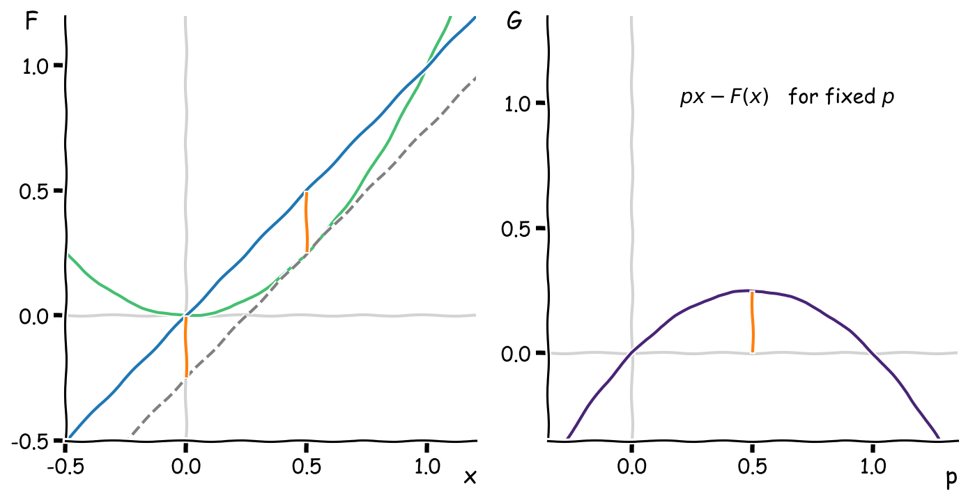
This gives us a second definition for the Legendre transform:

\[\boxed{G(p) = \max_x \{p\,x - F(x)\} \quad \text{for }F(x)\text{ convex up}}\]

Operationally, when calculating the maximum over \(x\), we’ll end up computing the derivative of the argument \(p\,x - F(x)\) and setting it to zero, which gives \(p = f(x)\) as before.

For concave down functions, the definition is \(G(p) = \min_x \{p\,x - F(x)\}\).

Now let’s have some fun.

Visual examples and curves which get us in trouble

I’ve worked out the Legendre transform in some common cases to give you a sense of how it behaves. Taking a function and translating the curve upwards shifts the Legendre transform downwards an equal amount:

Translating the original curve to the right shifts the Legendre transform to the left and downwards on a diagonal:

You can find a whole slew of properties of the Legendre transform on Wikipedia.

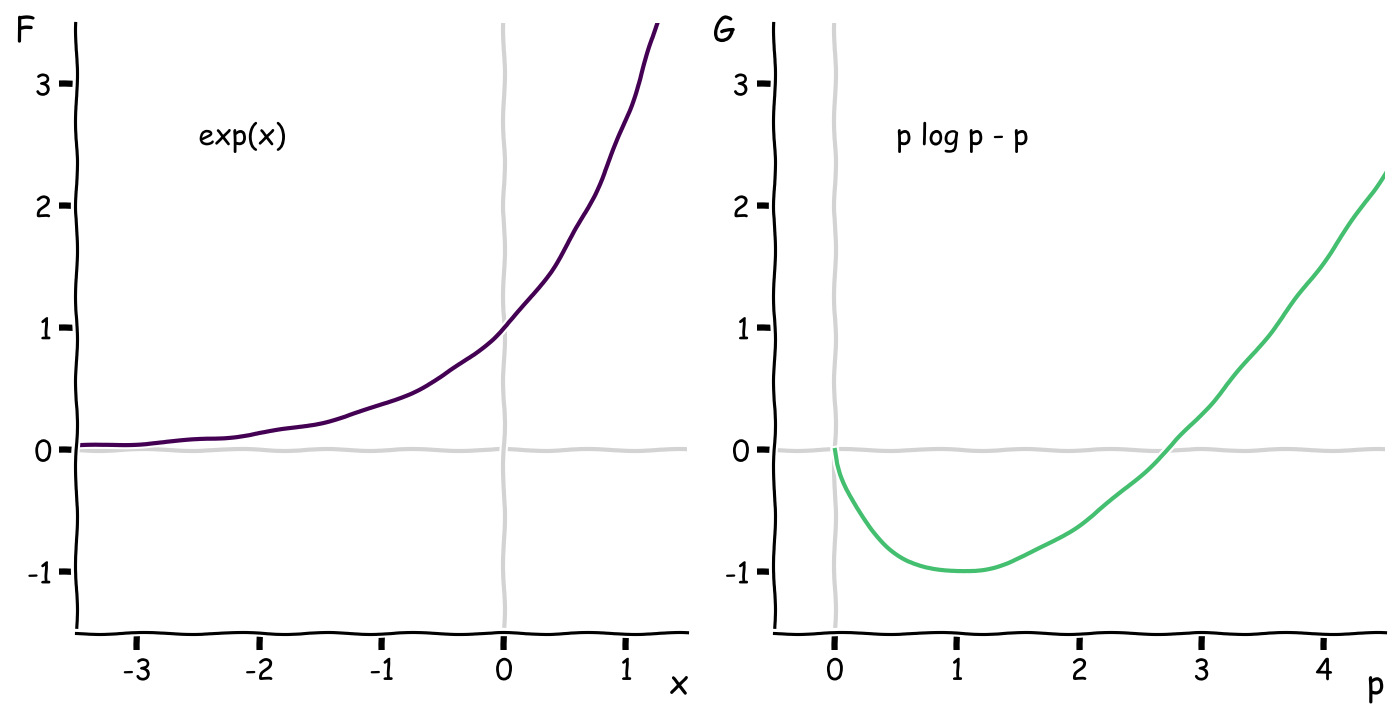
Moving away from parabolas, the transform of the exponential function \(e^x\) is only defined for \(p > 0\) because the slopes of the tangent lines are all positive.

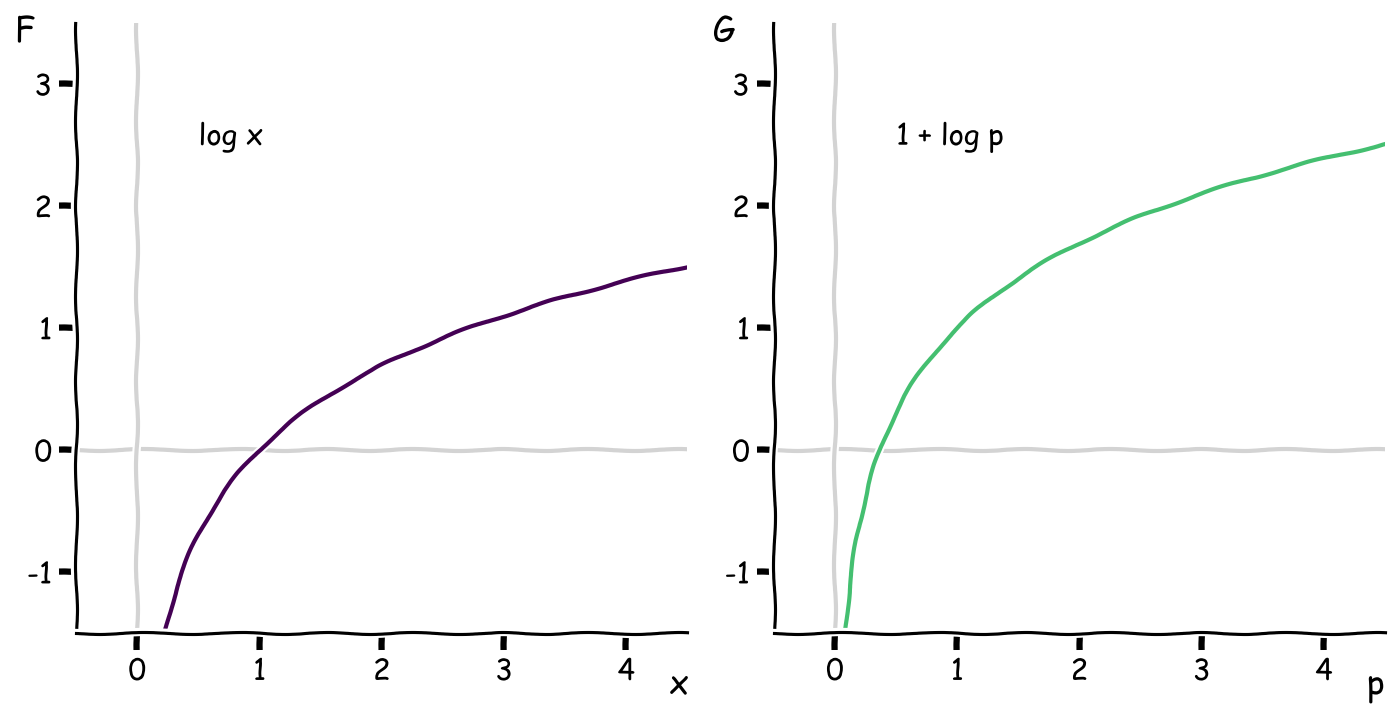
The transform of the (natural) logarithm is again a logarithm:

And for a fun one, the Legendre transform of a circle \(F(x) = \pm \sqrt{1-x^2}\) is the hyperbola \(G(p) = \mp \sqrt{1+p^2}\):

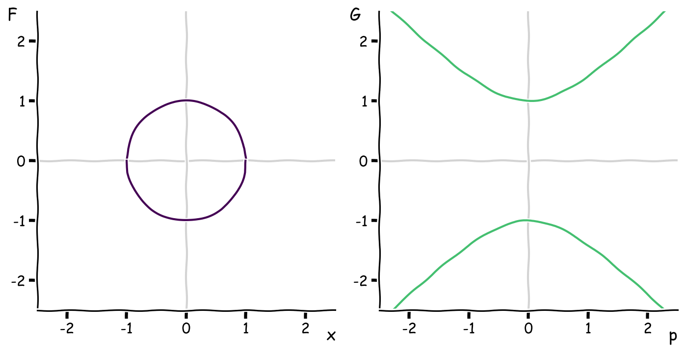
The top half of the circle corresponds to the bottom branch of the hyperbola, and vice versa.

I’ve been careful to choose curves that have well-behaved transforms. What kinds of curves have poorly-behaved Legendre transforms? Because the independent variable \(p\) in the transform is the slope of the tangent lines, you might guess that a function \(F(x)\) that is non-convex might behave poorly because multiple points have tangent lines with the same slope. Here’s an example: a double well.

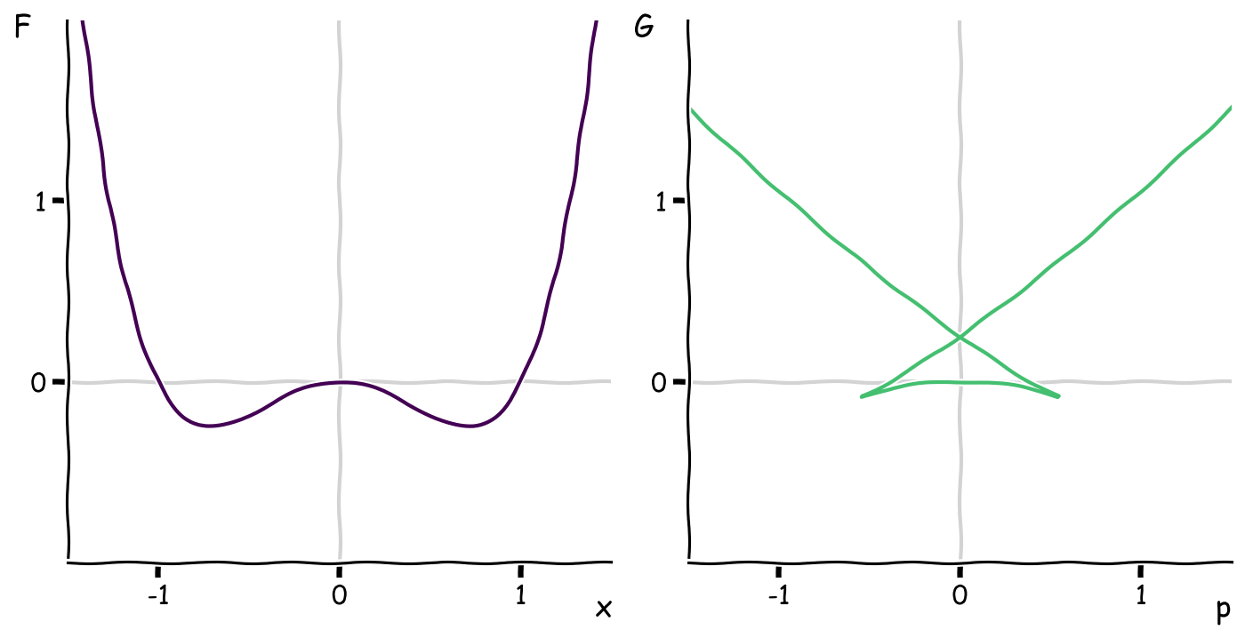
The Legendre transform (technically the Legendre-Fenchel transform in this more general case) becomes multi-valued. The two minima in \(F(x)\) map onto the “X” crossing on the vertical axes in the \(G(p)\) plot while the two cusps or “horns” in the transform correspond to the two points where \(F\) changes concavity.

As an aside, transforms of non-convex functions are related to convex hulls and the Maxwell construction, but to avoid these complexities, we’ll deal only with convex or concave functions going forward. Another way of saying this is that we’ll restrict ourselves to functions whose derivative is single-valued when considered as a function of \(p\). For our purposes, that means \(p = f(x)\) is monotonic increasing or decreasing.

The example on the left is fine. The example on the right is not permissible because there are some values of \(p\) which corresponds to multiple values of \(x\).

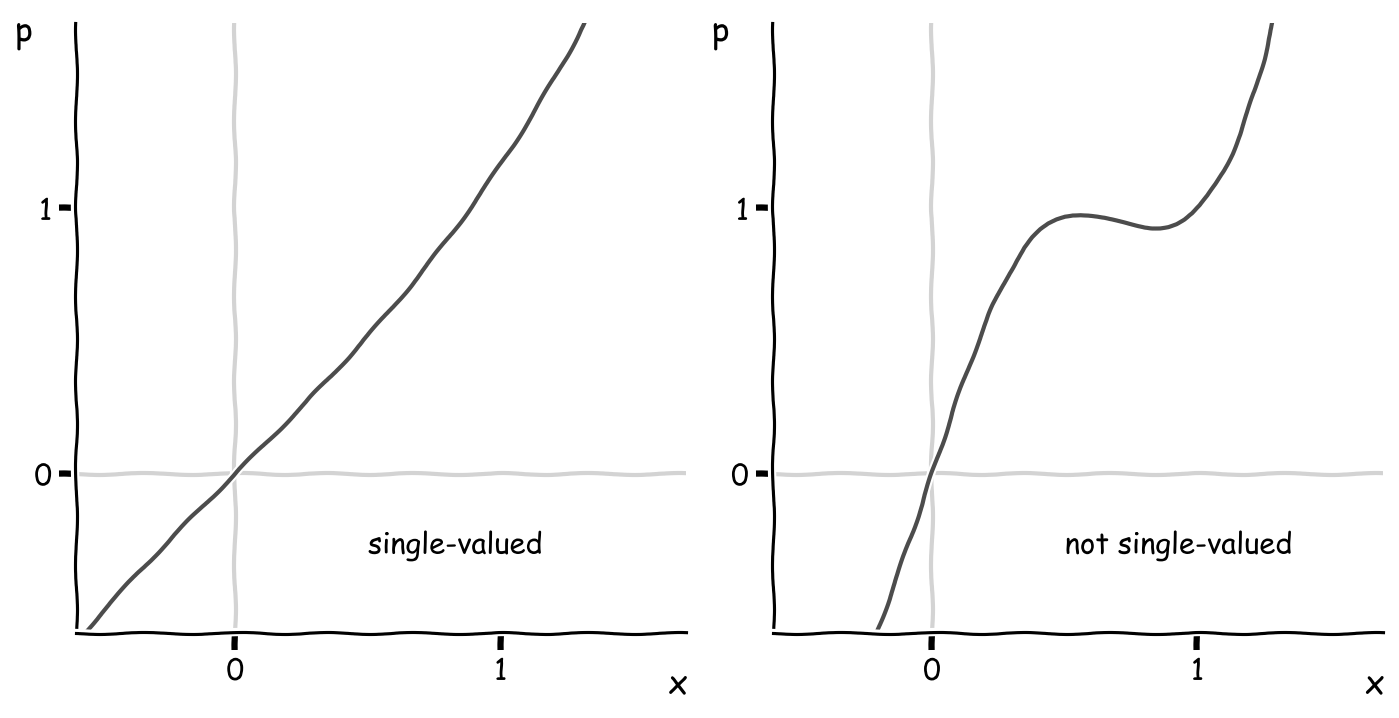
The fact that the derivative \(p = f(x)\) is single-valued means that it has an inverse \(x = g(p)\). Choosing \(p\) uniquely specifies \(x\), and either one could play the role as the independent variable.

Is the derivative \(g = G'\) of the Legendre transform equal to the inverse of \(f\), as the notation suggests?

See the next section!

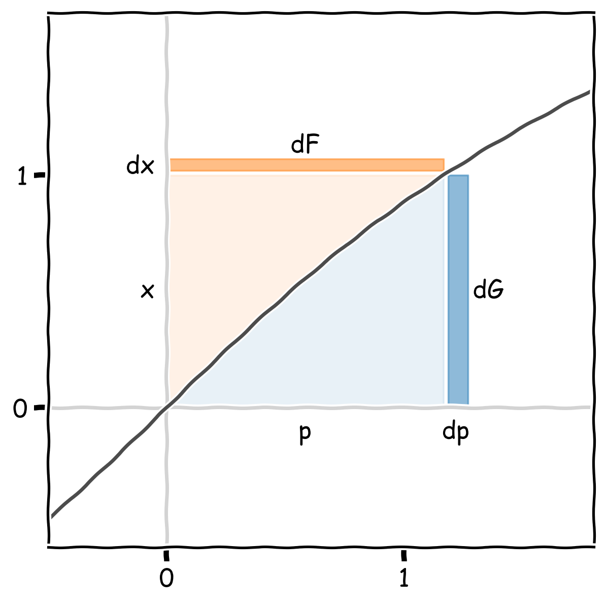
In the past three sections, we’ve explored the Legendre transform from the perspective of duality for plane curves: the mapping between points and tangent lines. In the following, I want to move from derivatives to integrals and reinterpret the construction in terms of areas. This will give us a beautifully symmetric view on the Legendre transform and lead to a connection to integrals of inverse functions.

From slopes to areas

Go back to the triangle in the plot of \(F(x)\) constructed by picking a point \(x\) and drawing the tangent line, which led to the relationship

\[p\,x = F + G\]

Each of the three terms is a length, and the equation essentially is two ways to express the height of the triangle: “the height of the triangle is equal to the slope \(p\) times the width \(x\), or equivalently, the sum of the line segments \(F\) and \(G\)”.

Now switch to the plot the derivative \(p = f(x)\). What does the triangle (specifically the height of the triangle) become?

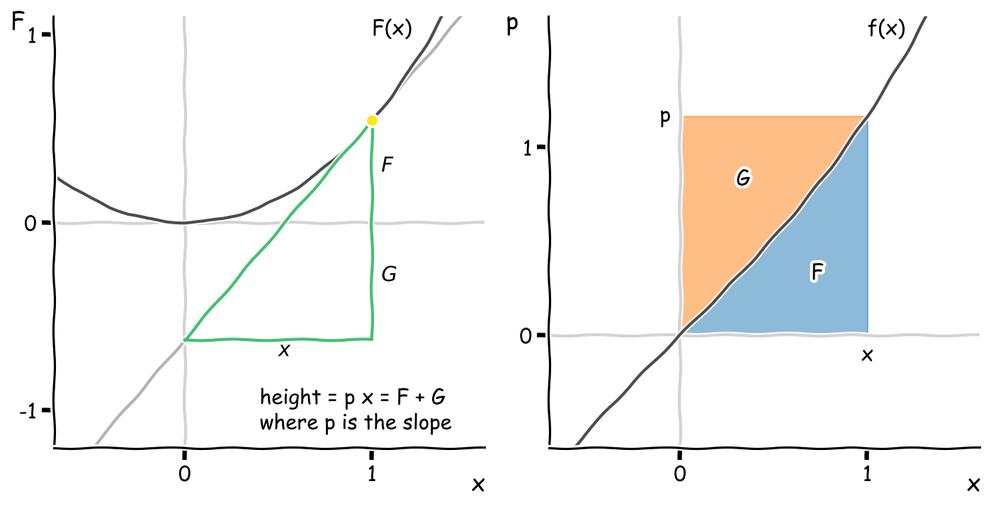
In the \(p\)-\(x\) axes, the three terms representing lengths become areas:

1. The height of the triangle \(p \, x\) becomes a rectangle with dimensions \(x \times p\).

2. The value \(F(x)\) becomes the area under the curve \(f\) integrated up to \(x\):

   \[F(x) = \int_0^x\! dx\, f(x)\]

3. To make things add up, the area above the curve \(f\) must be the Legendre transform \(G\)!

This area diagram will give us the equation for the Legendre transform: to express the area \(G\) as a function of \(p\), use the fact that the derivative \(p = f(x)\) is single-valued and view the curve in terms of its inverse \(x = g(p)\). I’ve flipped the axes and plotted the inverse below on the left:

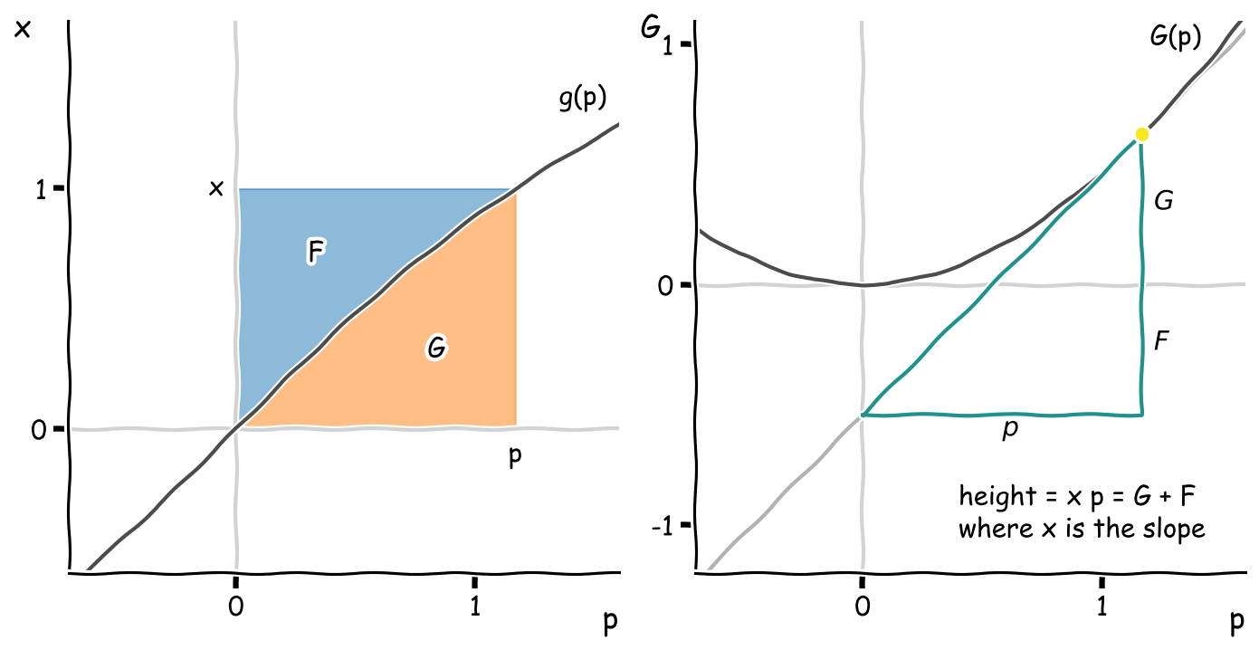
The area under the curve up to \(p\) is:

\[G(p) = p\,g(p) - F(g(p))\]

which is the Legendre transform. In terms of areas, the symmetry between \(F\) and \(G\) is beautifully explicit: they are the two partitions of a rectangle defined by the derivative curve \(f(x)\), or equivalently, \(g(p)\).

The area diagram answers another question we hinted at earlier: how are the derivatives of \(F\) and \(G\) related? They are inverses! Mathematically, the area under the curve is the integral

\[G(p) = \int_0^p\! dp\, g(p)\]

which means the derivative \(g(p) = G'(p)\) is indeed the inverse of \(f(x) = F'(x)\), as promised.

Physicists will often abuse notation and write the duality between the derivatives as

\[\boxed{ \begin{align} \frac{dF}{dx} &= p \\ \frac{dG}{dp} &= x \end{align} }\]

Yes, it doesn’t tell you when \(p\) and \(x\) are acting as functions or as variables, but the equations sure are symmetric! This duality is useful because it allows us to construct families of potentials in physical applications. For a system, if \(x\) is the independent variable

I’ve simplified the arguments by choosing a function \(F(x)\) which both passes through the origin and has zero slope at the origin. You can check that a suitably modified construction, involving keeping track of the constant of integration and the integration limits, continues to work for more general functions satisfying neither of those conditions.

I can’t pass up showing you one more surprising connection the Legendre transform has to integral calculus before moving to physics.

Integration of inverse functions

Back in 1905, the mathematician Charles-Ange Laisant published a short article titled “Integration of Inverse Functions”. In it, he posed a simple question: given a function \(y = f(x)\) which has an inverse \(x = g(y)\), what is the integral of \(g\)?

Given the simplicity of the question, he wrote that he “could hardly believe that this theorem is new.” Defining \(F(x) = \int dx\, f(x)\) and \(G(x) = \int dx\, g(x)\), Laisant showed that

\[G(x) = x\, g(x) - F(g(x))\]

Look familiar?! In fact, among the three proofs he provided, his graphical proof is based on the area construction we discussed above. From this viewpoint, the Legendre transform of a function is the integral of the inverse of its derivative.

Another of the proofs provided by Laisant uses integration by parts:

\[\int\! f(x)\, dx = x\, f(x) - \int\! x\, df(x) = x\, f(x) - \int\! g(p)\, dp\]

where we eliminated the differential \(df\) by substituting \(p = f(x)\) in the second integral and used \(x = g(p)\). Using the notation for the antiderivatives:

\[F(x) = x\, f(x) - G(p) = x\, f(x) - G(f(x))\]

which is the same formula above.

Here’s an example of the formula in action. Given:

\[\newcommand{\arctanh}{\mathop{\rm arctanh}\nolimits} f(x) = \tanh x, \qquad g(x) = \arctanh x, \qquad F(x) = \log\cosh x\]

straightforward substitution gives

\[G(x) = x\, \arctanh x - \log\cosh\arctanh x = x\, \arctanh x + \frac{1}{2} \log (1-x^2)\]

where we used \(\cosh\arctanh x = 1 / \sqrt{1-x^2}\).

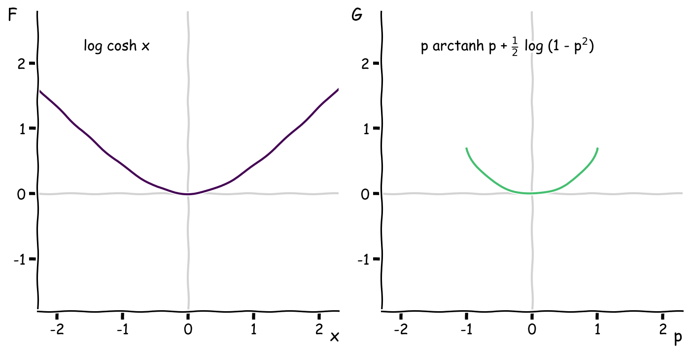
The domain of the transform is restricted to \([-1, 1]\) because \(F\) has asymptotes with slope \(p = \pm 1\).

To conclude these sections on mathematics, I hope you’ve discovered that the Legendre transform is actually rather pedestrian and requires nothing more than basic calculus to understand, yet provides insight into the tangents of plane curves and the connections between core elements of calculus. It’s properties naturally find application in physics, which we turn to next.

Potentials and their derivatives

In classical mechanics, we often want to know how a system will respond when we apply some perturbation. For example, given a spring, what is the restoring force when we stretch it an amount \(x - x_0\) away from its equilibrium length? The experimentally determined relationship in the linear regime is \(F = -k\,(x-x_0)\), termed Hooke’s law.

However, another way to answer this question is to introduce the concept of a potential energy \(V(x)\) whose derivative with respect to \(x\) tells us the force:

\[F(x) = -\frac{dV(x)}{dx}\]

For the case of a spring with spring constant \(k\), the potential energy is \(V(x) = k(x-x_0)^2/2\).

Note: the convention in physics is to compute the force of the potential acting on the object, so there’s an extra minus sign floating around which we’ll need to keep track of.

What if I wanted to construct a potential \(W(F)\) whose derivative with respect to the force \(F\) experienced by the object gives us the displacement \(x\)?

Use the derivative properties of the Legendre transform: the relationship between the potential energy and force is just the first relation with the substitutions \(f \rightarrow -V\) and \(p \rightarrow F\). Substituting \(g \rightarrow -W\) in the second relation gives:

\[x(F) = -\frac{dW(F)}{dF}\]

The potential \(W\) is the Legendre transform of \(V\), up to some minus signs! The answer for the mass attached to a spring is

\[W = \frac{F^2}{2k} - Fx_0\]

What physical quantity does \(W\) measure? It has units of energy, and it is the Legendre transform of the potential energy, so \(W\) must be something related to the potential energy (and not, e.g. related to the kinetic energy).

The Legendre transform allows us to construct a potential where the perturbing and reponse variables are swapped. In this example, the original perturbing (also called the control or independent) variable \(x\) is replaced in favor of the response variable \(F\). Control-response pairs occur in many physics, and when they satisfy [XYZ] condition, they are termed conjugate variables.

Lagrangians and Hamiltonians

For students of analytical mechanics, one of the first concepts introduced is that of a Lagrangian, which is the kinetic \(T\) minus the potential \(V\) energy, written as a function of the coordinates \(q_i(t)\) and velocities \(\dot{q}_i(t)\).

steps is to derive the Lagrangian by imagining small displacements in the coordinates of a system. The result is a functional that takes as input a function

---

How do differentials behave? Imagine making a small change \(dx\)

Imagine making a small change in the height of the triangle \(d(px)\). Using the product rule gives \(d(px) = p\,dx + x\,dp\)

---

It turns out a useful quantity to examine is the derivative of \(g(p)\). A straightforward calculation gives the answer:

\[\begin{align} \frac{dg}{dp} &= \frac{d}{dp} [ p\,x(p) - f(x(p)) ] \\ &= x(p) + p \, \frac{dx}{dp} - \frac{df}{dx} \frac{dx}{dp} \\ &= x(p) \end{align}\]

The derivative of the Legendre transform is the original independent variable \(x\).

Going back to differentials, what happens when we have a function \(f(x,y)\) of multiple variables and transform just one of them?

\[df = p\,dx + q\,dy\] \[dg = x\,dp - q\,dy\]

The second term acquires a minus sign. The spectator variables aren’t left alone (why is this important?). Example:

\[f(x, y) = x^2 + y^2\] \[g(p, y) = \frac{p^2}{4} - y^2\]

We went from a paraboloid to a hyperbolic paraboloid. Again, why is this important?

\[df + dg = p\,dx + x\,dp\]

[Relationship with Laplace transform via saddle point]

xBehavior of differentials:

\[df = p \, dx \quad \text{where } p = \frac{df}{dx}\]

What about the differential of \(g\)?

\[dg = x\,dp + p \frac{dx}{dp} - \frac{df}{dx} \frac{dx}{dp}\]

The last two terms cancel, and we find

\[dg = x\,dp\]

Point is the slope of the Legendre transform is the original independent variable \(x\).

Maximizing entropy

For students of thermodynamics, you may remember being introduced to a quantity called the Helmholtz free energy, \(F = E - TS\), and being told it is the Legendre transform of the energy \(E\). What does this quantity physically measure and why is it related to energy by a Legendre transform?

What is entropy? Define entropy: it’s the number of states compatible with macroscopic constraints. Empirically, it’s also a ratio of heat flow to temperature. Consider bringing up entropy tables.

Assume the 2nd law of thermodynamics: that a system will evolve in such a way to maximize it’s entropy.

Given the classic set up of a system \(A\) and a much bigger reservoir \(B\), what division of energy between the two parts maximizes entropy? Imagine we start off with all the energy in \(B\) and none in \(A\). No energy in \(A\) means its contribution to the entropy is zero, so

\[S_\text{tot} = S_B(E_\text{tot})\]

As we allow energy \(E\) to flow from \(B\) to \(A\), the entropy of \(B\) will decrease while the entropy of \(A\) increases.

\[S_\text{tot}(E, E_\text{tot}) = S_A(E) + S_B(E_\text{tot} - E)\]

How much does the entropy of \(B\) decrease by? Taylor expand:

\[S_B(E_\text{tot} - E) \approx S_B(E_\text{tot}) - E \left. \frac{\partial S_B}{\partial E} \right|_{E = E_\text{tot}}\]

We call the slope of the reservoir’s entropy \(\beta(E)\), the inverse temperature.

\[\Delta S_\text{tot}(E) = S_A(E) - E \, \beta(E)\]

Where \(\Delta S_\text{tot}(E) = S_\text{tot}(E, E_\text{tot}) - S_B(E_\text{tot})\). The right hand side is the Legendre transform of the entropy of \(A\).

Because for a big system, its entropy is nearly linear in the energy, the maximization of total entropy leads to the Legendre transform.

\[\Delta S_\text{tot}(\beta) = S_A(E(\beta)) - E(\beta) \, \beta\]

The Legendre transform of the entropy tells us how much the entropy will be produced when bringing the system from absolute zero to \(T = 1 / \beta\).

What does the Helmholtz free energy physically correspond to? The quantity \(\beta F\) is the total amount of entropy produced when bringing the system from absolute zero to its final equilibrium temperature when placed in contact with the resevoir.

Why is it’s slope something we feel as hot and cold? Think about if we felt total energy instead of temperature: we’d find the Earth unbearable.

Why are thermodynamic conventions different than the symmetric mathematical presentation we chose above?

What is an example of this maximization in action? Example of gas piston with spring. [Wait, doesn’t this involve a change in volume?]

Notes

Questions:

• How does Legendre transforms relate to derivatives and conjugate pairs? What about units?

• What’s wrong with using \(F(x(p))\), where \(p = dF(x)/dx\)?

• What is the differential form of the Legendre transform? How does it relate to integration by parts or the product rule?

• Ex: classical mechanics

  • What does the Legendre transform of a potential \(V(x)\) mean?

  • Both have units of energy: what energy is it?

• Ex: Hamiltonian mechanics

  • Why does the Legendre transform show up?

• Ex: Thermodynamics:

  • Why does the Legendre transform show up? How is this related to Laplace transforms?

  • How do Legendre transforms relate to the Gibb’s construction?

  • What is the physical meaning of the Legendre transforms? What is the Helmholtz “free” energy?

  • How are Legendre transforms related to entropy maximization and free energy minimization?

Answered:

• What is the Legendre transform intuitively?

• How is the Legendre transform expressed mathematically? How are the supremum and \(G + F = xy\) expressions related?

• What are useful mathematical properties of the Legendre transform? Why is the Legendre transform an involution?

• Why is there a convexity constraint?

Writer’s notes:

• Show, don’t tell. Sentences like “The legendre transform is so fundamental that it is one of those ideas which have many viewpoints, each of which highlights one aspect of the idea” are fluff and convey little information. Instead, get straight to the point by asking a question, then immediately answering it.

• Directly introduce new ideas. Introducing ideas by pointing to how current teaching screws it up complicates the exposition. The student needs to mentally jump through two steps rather than one.

Resources

Clare Yu notes: lectures 13-16.

Zia AJP article

Munger: mathematical exposition based on product rule

StackExchange: nice graphical representation of \(F + G = xy\) and requirement of maintaining variational principles under change of conjugate variable pairs.

Manton: dense math, maybe not useful.

Fast Legendre transform: viewpoint from image analysis

Supporting hyperplane

Deserno: mathematical exposition noting information content of functions

Notes on canonical ensemble

Adiabatic processes for ideal gas

Entropy changes in an ideal gas

Heat capacities of gases: notes for constant volume vs. constant pressure

P-v-T: PvT diagrams for models of gases with varying degrees of realism

Canonical ensemble: formulas for ideal gas in microcanonical and canonical ensembles

Free energy: lecture notes providing concrete worked example of Helmholtz free energy for system with a spring connected to a gas piston.

Zia Legendre transform presentation