A human heart is an astounding machine that is designed to continually function for up to a century without failure. One of the key ways to measure how well your heart is functioning is to compute its ejection fraction: after your heart relaxes at its diastole to fully fill with blood, what percentage does it pump out upon contracting to its systole? The first step of getting at this metric relies on segmenting (delineating the area) of the ventricles from cardiac images.

During my time at the Insight AI Program in NYC, I decided to tackle the right ventricle segmentation challenge from the calls for research hosted by the AI Open Network. I managed to achieve state of the art results with over an order of magnitude less parameters; below is a brief account of how.

Problem description

From the call for research:

Develop a system capable of automatic segmentation of the right ventricle in images from cardiac magnetic resonance imaging (MRI) datasets. Until now, this has been mostly handled by classical image processing methods. Modern deep learning techniques have the potential to provide a more reliable, fully-automated solution.

All three winners of the left ventricle segmentation challenge sponsored by Kaggle in 2016 were deep learning solutions. However, segmenting the right ventricle (RV) is more challenging, because of:

[the] presence of trabeculations in the cavity with signal intensities similar to that of the myocardium; the complex crescent shape of the RV, which varies from the base to the apex; difficulty in segmenting the apical image slices; considerable variability in shape and intensity of the chamber among subjects, notably in pathological cases, etc.

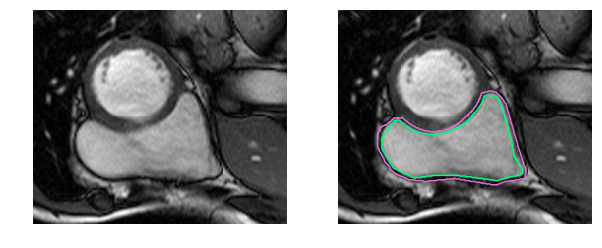
Medical jargon aside, it’s simply more difficult to identify the RV. The left ventricle is a thick-walled circle while the right ventricle is an irregularly shaped object with thin walls that sometimes blends in with the surrounding tissue. Here are the manually drawn contours for the inner and outer walls (endocardium and epicardium) of the right ventricle in an MRI snapshot:

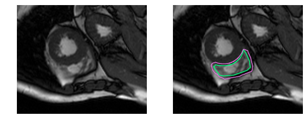
That was an easy example. This one is more difficult:

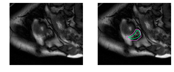
And this one is downright challenging to the untrained eye:

Human physicians in fact take twice as long to determine the RV volume and produce results that have 2-3 times the variability as compared to the left ventricle [1]. The goal of this work is to build a deep learning model that automates right ventricle segmentation with high accuracy. The output of the model is a segmentation mask, a pixel-by-pixel mask that indicates whether each pixel is part of the right ventricle or the background.

The dataset

The biggest challenge facing a deep learning approach to this problem is the small size of the dataset. The dataset (accessible here) contains only 243 physician-segmented images like those shown above drawn from the MRIs of 16 patients. There are 3697 additional unlabeled images, which may be useful for unsupervised or semi-supervised techniques, but I set those aside in this work since this was a supervised learning problem. The images are 216\(\times\)256 pixels in size.

Given the small dataset, one would suspect generalization to unseen images would be hopeless! This unfortunately is the typical situation in medical settings where labeled data is expensive and hard to come by. The standard procedure is to apply affine transformations to the data: random rotations, translations, zooms and shears. In addition, I implemented elastic deformations, which locally stretch and compress the image [2].

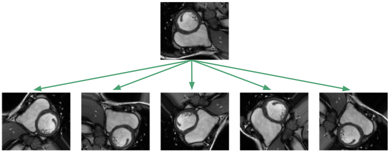
The goal of such augmentations is to prevent the network from memorizing just the training examples, and to force it to learn that the RV is a solid, crescent-shaped object that can appear in a variety of orientations. In our training framework, we apply the transformations on the fly so the network sees new random transformations during each epoch.

As is also common, there is a large class imbalance since most of the pixels are background. Normalizing the pixel intensities to lie between 0 and 1, we see that across the entire dataset, only 5.1% of the pixels are part of the RV cavity.

In constructing the loss functions, I experimented with reweighting schemes to balance the class distributions, but ultimately found that the unweighted average performed best.

During training, 20% of the images were split out as a validation set. The organizers of the RV segmentation challenge have a separate test set consisting of another 514 MRI images derived from a separate set of 32 patients, for which I submitted predicted contours for final evaluation.

Let’s look at model architectures.

U-net: the baseline model

Since we only had a 4 week timeframe to complete our projects at Insight, I wanted to get a baseline model up and running as quickly as possible. I chose to implement a u-net model, proposed by Ronneberger, Fischer and Brox [3], since it had been quite successful in biomedical segmentation tasks. U-net models are promising, as the authors were able to train their network with only 30 images by using aggressive image augmentation combined with pixel-wise reweighting. (Interested readers: here are reviews for CNN [4] and conventional [5] approaches.)

The u-net architecture consists of a contracting path, which collapses an image down into a set of high level features, followed by an expanding path which uses the feature information to construct a pixel-wise segmentation mask. The unique aspect of the u-net are its “copy and concatenate” connections which pass information from early feature maps to the later portions of the network tasked with constructing the segmentation mask. The authors propose that these connections allow the network to incorporate high level features and pixel-wise detail simultaneously.

The architecture we used is shown here:

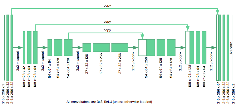
We adapted the u-net to our purposes by reducing the number of downsampling layers in the original model from four to three, since our images were roughly half the size as those considered by the u-net authors. We also zero pad our convolutions (as opposed to unpadded) to keep the images the same size. The model was implemented in Keras.

The u-net did not take long to implement and benchmark, so there was time to explore novel architectures. I’ll present the two other architectures I developed before jumping to aggregated results for all three models.

Dilated u-nets: global receptive fields

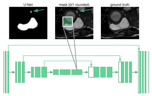
Segmenting organs requires some knowledge of the global context of how organs are arranged relative to one another. It turned out that the neurons in even the deepest part of the u-net only had receptive fields that spanned 68\(\times\)68 pixels. No part of the network could “see” the entire image and integrate global context in producing the segmentation mask. The reasoning is that the network would have no understanding that there is only one right ventricle in a human. For example, it misclassifies the blob marked with an arrow in the following image:

Rather than adding two more downsampling layers at the cost of a huge increase in network parameters, we use dilated convolutions [6] to increase the receptive fields of our network.

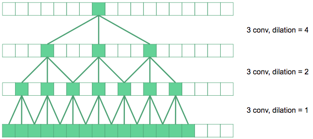
Dilated convolutions space out the pixels summed over in the convolution by a dilation factor. In the diagram above, the convolutions in the bottom layer are regular 3\(\times\)3 convolutions. The next layer up, we have dilated the convolutions by a factor of 2, so their effective receptive field in the original image is 7\(\times\)7. The top layer convolutions are dilated by 4, producing 15\(\times\)15 receptive fields. Dilated convolutions produce exponentially expanding receptive fields with depth, in contrast to linear expansion for stacked conventional convolutions.

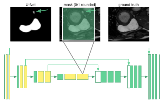
Schematically, we replace the convolutional layers producing the feature maps marked in yellow with dilated convolutions in our u-net. The innermost neurons now have receptive fields spanning the entire input image. We call this a “dilated u-net”.

Dilated densenets: multiple scales at once

For segmentation tasks, we need both global context and information from multiple scales to produce the pixel-wise mask. What if we only used dilated convolutions to generate global context, rather than downsampling to “smash” the image down to a small height and width? Now that the convolutional layers all have the same size, we could use “copy and concatenate” connections between all the layers:

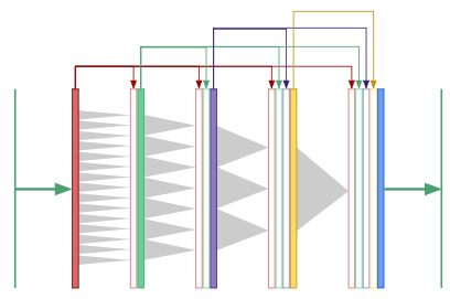
This is a “dilated densenet”, which combines two ideas: dilated convolutions and densenets, which were developed by Huang, et. al. [7].

In densenets, the output of the first convolutional layer is fed as input into all subsequent layers, and similarly with the second, third, and so forth. The authors show that densenets have several advantages:

they alleviate the vanishing-gradient problem, strengthen feature propagation, encourage feature reuse, and substantially reduce the number of parameters.

At publication, densenets had surpassed the state of the art on the CIFAR and ImageNet classification benchmarks.

However, densenets have a serious drawback: they are extremely memory intensive since the number of feature maps grow quadratically with network depth. The authors used “transition layers” to cut down on the number of feature maps midway through the network in order to train their 40, 100 and 250 layer densenets. Dilated convolutions eliminates the need for such deep networks and transition layers since only 8 layers are needed to “see” an entire 256\(\times\)256 image.

In the final convolutional layer of a dilated densenet, the neurons have access to global context as well as features produced at every prior scale in the network. In our work, we use an 8-layer dilated densenet and vary the growth rate from 12 to 32. Here’s the astounding aspect: the dilated densenet is extremely parameter efficient. Our final model uses only 190K parameters, a point we’ll come back to when discussing results.

Let’s look at how to train these models, and then move on to their performance in segmenting right ventricles.

Training: what loss and hyperparameters to use?

We need a way to measure model performance quantitatively during training. The organizers of the segmentation challenge chose to use the dice coefficient. The model will output a mask \(X\) delineating what it thinks is the RV, and the dice coefficient compares it to the mask \(Y\) produced by a physician via:

\[\mathrm{dice}(X, Y) = \frac{2 X \cap Y}{X + Y}\]

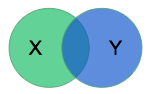
The metric is (twice) the ratio of the intersection over the sum of areas. It is 0 for disjoint areas, and 1 for perfect agreement. (The dice coefficient is also known as the F1 score in the information retrieval field since we want to maximize both the precision and recall.) In the rest of this section, various technical details of the training methodology are provided — feel free to skip to the results section.

We used the standard pixel-wise cross entropy loss, but also experimented with using a “soft” dice loss. Denote by \(\hat{y}_{nk}\) the output of the model, where \(n\) runs over all pixels and \(k\) runs over the classes (in our case, background vs. right ventricle). The ground truth masks are one-hot encoded and denoted by \(y_{nk}\).

For the pixel-wise cross entropy, we include weights \(w_k\) to allow for reweighting the strongly imbalanced classes:

\[L(y, \hat{y}) = -\sum_{nk} w_k y_{nk} \log \hat{y}_{nk}\]

Simple averaging corresponds to \(w_\mathrm{background} = w_\mathrm{RV} = 0.5\). We experimented with \(w_\mathrm{background} = 0.1\) and \(w_\mathrm{RV} = 0.9\) to bias the model to pay more attention to the RV pixels.

We also use a “soft” dice loss summed over the classes, again with weights \(w_k\) to allow for rebalancing:

\[L(y, \hat{y}) = 1 - \sum_k w_k \frac{\sum_n y_{nk} \hat{y}_{nk}}{\sum_n y_{nk} + \sum_n \hat{y}_{nk}}\]

We take one minus the dice coefficient so the loss tends towards zero. This dice coefficient is “soft” in the sense that the output probabilities at each pixel \(\hat{y}_{nk}\) aren’t rounded to be \([\hat{y}_{nk}] \in \{0, 1\}\). Rounding isn’t a differentiable operation and cannot be used as a loss function. We use the usual “hard” dice coefficient to report the classification performance.

In our training runs, we varied the following hyperparameters:

• Batch normalization
• Dropout
• Learning rate
• Growth rate (for the dilated densenets)

For the final results shown below, we used the adam optimizer with the default initial learning rate of \(10^{-3}\) and trained for 500 epochs. Each image in the dataset was individually normalized by subtracting its mean and dividing by its standard deviation. We used the unweighted pixel-wise cross entropy as the loss function, as it performed better than the weighted and dice losses. Dropout was turned off as it actually degraded validation performance. Pre-activation batch normalization was used only for the dilated densenet, as batch normalization reduced performance for the u-net and dilated u-net. The dilated densenet had a growth rate of 24, which was a good balance between model performance and size. We used a batch size of 32, except for the dilated densenet, which required a batch size of 3 on our 16GB GPU due to memory constraints.

Results

Andrew Ng explains in this useful talk that having an estimate of human performance provides a roadmap for how to evaluate model performance. Researchers estimated that humans achieve dice scores of 0.90 (0.10) on RV segmentation tasks (we write the standard deviation in parentheses) [8]. The leading published model is a fully convolutional network (FCN) by Tran [9] with 0.84 (0.21) accuracy on the test set.

The u-net baseline achieves a dice score of 0.91 (0.06) on the training set, which means the model has little bias and the capacity to perform at human-level. However, the validation accuracy is 0.82 (0.23), indicating a large variance. As Andrew states, this can be dealt with by getting more data (not possible), regularization (dropout and batch normalization did not help), or trying a new model architecture.

This led to an examination of edge cases, an understanding of receptive fields, and ultimately the dilated u-net architecture. It beats the original u-net and achieves 0.92 (0.08) on the training set and 0.85 (0.19) on the validation set.

Finally, dilated densenets were loosely inspired by the similarity between dilated convolutions and tensor networks used in physics. This architecture achieves 0.91 (0.10) on the training set and 0.87 (0.15) on the validation set with only 0.19M parameters.

The final test required submitting the segmentation contours produced by the models for evaluation on the test set held out by the organizers of the RV segmentation challenge. The dilated u-net beats the state of the art and the dilated densenet is close behind even though it has ~20\(\times\) less parameters!

The results are summarized in the following tables. The values are the dice coefficients, along with their uncertainties in parentheses. The state of the art are bolded. For the endocardium:

Method	Train	Val	Test	Params
Human	–	–	0.90 (0.10)	–
FCN (Tran 2017)	–	–	0.84 (0.21)	~11M
U-net	0.91 (0.06)	0.82 (0.23)	0.79 (0.28)	1.9M
Dilated u-net	0.92 (0.08)	0.85 (0.19)	0.84 (0.21)	3.7M
Dilated densenet	0.91 (0.10)	0.87 (0.15)	0.83 (0.22)	0.19M

For the epicardium:

Method	Train	Val	Test	Params
Human	–	–	0.90 (0.10)	–
FCN (Tran 2017)	–	–	0.86 (0.20)	~11M
U-net	0.93 (0.07)	0.86 (0.17)	0.77 (0.30)	1.9M
Dilated u-net	0.94 (0.05)	0.90 (0.14)	0.88 (0.18)	3.7M
Dilated densenet	0.94 (0.04)	0.89 (0.15)	0.85 (0.20)	0.19M

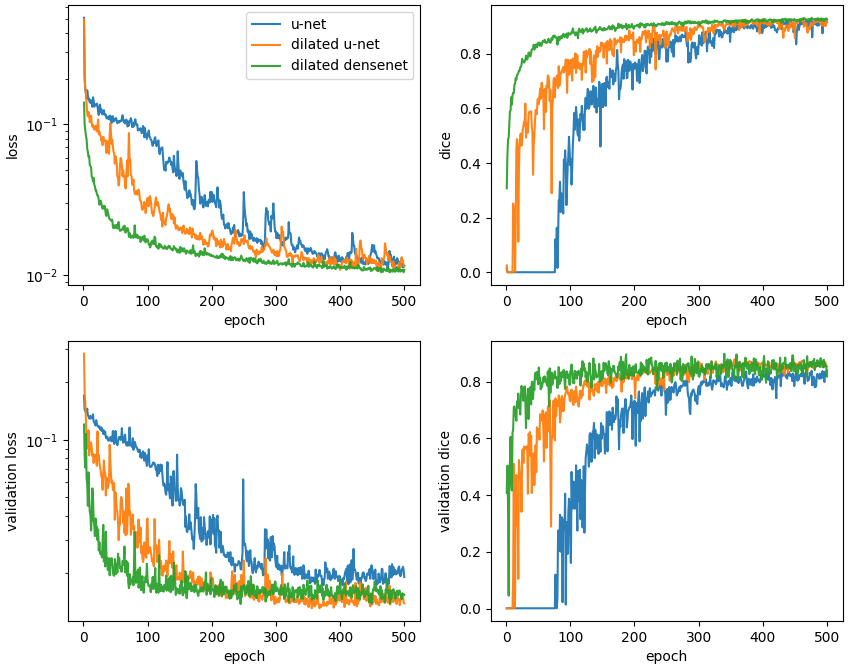
Typical learning curves are shown below. In all cases, the validation loss plateaus and does not exhibit an upturn characteristic of overfitting. On a per epoch basis, it is astounding to see how quickly the dilated densenet learns relative to the u-net and dilated u-net.

Returning to cardiac segmentation, in our results, as well as in the published literature, the dice scores exhibit large standard deviations. Boxplots show that for some images, the networks struggle to segment the RV to any extent:

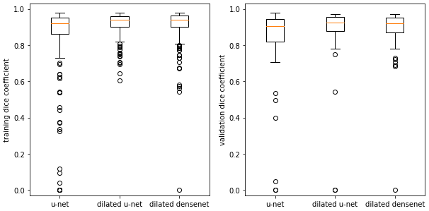
Examining the outliers, we find they mostly arise from apical slices (near the bottom tip) of the heart where the RV is difficult to identify. This is an outlier for the dilated densenet on the validation set:

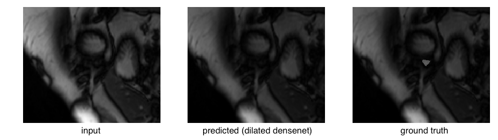
The right ventricle is barely visible in the original image and the ground truth mask is quite small in area. Compare that to a relatively successful segmentation:

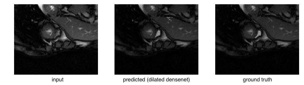
or even an easy case:

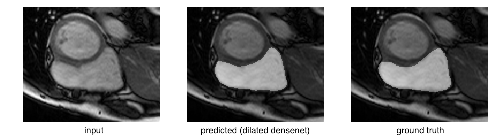
Considering these edge cases, it’s clear that a big challenge facing these models lies in eliminating catastrophic failures, as they would lead to skewed cardiac volumes. Focusing on reducing the standard deviation by eliminating these outliers will raise the mean dice scores.

Summary and future directions

The performance of deep learning models can sometimes seem magical, but they are the result careful engineering. Even in regimes with small datasets, well-selected data augmentation schemes allow deep learning models to generalize well. Reasoning through how data flows through a model leads to architectures well-matched to the problem domain. Following these ideas, we were able to create models that achieve state of the art for segmenting the right ventricle in cardiac MRIs. I’m especially excited to see how dilated densenets will perform on other image segmentation benchmarks and explore permutations of its architecture.

I’ll end with some thoughts for the future:

• Reweight the dataset to emphasize the difficult to segment apical slices.
• Explore quasi-3D models where the entire stack of registered cardiac slices are simultaneously fed into the model.
• Explore multistep (localization, registration, segmentation) pipelines.
• Optimize for the ejection fraction, the final figure of merit, in a production system.
• Memory-efficient dilated densenets: densely connected networks are notorious for requiring immense amounts of memory. The raw TensorFlow is particularly egregious, limiting us to 8 layers with a batch size of 3 images on a 16GB GPU. Switching to the recently-proposed memory efficient implementation [10], would allow for deeper architectures.

About this project

The Insight AI Fellows Program is an intense, 7-week experience where fellows already possessing deep technical expertise are provided an environment to bridge the small skills gap needed to enter the AI field. A major component of bridging that gap involves completing a project in deep learning in order to gain hands-on experience in AI.

As a relative novice to deep learning, I approached project selection like a new graduate student: choose a clearly motivated and well scoped problem that could be tackled in 4 weeks. I deliberately selected a project with small a dataset to allow me to quickly iterate and gain experience. This project met those goals and provided the intellectual playground to create dilated densenets.

The code is available on github.