
Company tagging
Let’s say you are an analyst and you want to know the fraction of companies which discuss carbon emissions in their public documents. How would you do it?
Background
The naive way: assemble a team of analysts to read all public documents from the universe of companies and make a determination of whether carbon emissions is discussed. If any paragraph in the set of documents published by a company discusses carbon emissions, then the analyst would add that company to the tally. At the end, divide the tally by the total number of companies to arrive the desired proportion.
In reality, you’re interested in multiple topics, from methane emissions to diversity initiatives to new funding, so the number of topics you want to tally up are in the hundreds. Combined with the size of the universe of documents (tens of thousands), the manual approach translates to millions of paragraphs which need to be scanned for hundreds of topics. Building a machine learning pipeline seems like a good idea: use a model to tag each paragraph as relevant or irrelevant to a given topic, then aggregate those binary tags together to make a per-company determination.
There is one big hurdle to building ML pipelines for tagging text: the problem is extremely imbalanced. The probability of any given paragraph being relevant to a topic is usually less than 1%, and often less than 0.1%. One way I’ve seen these problems solved is with a two-step pipeline: a rule-based search query to to select candidate paragraphs, followed by a deep learning model which performs paragraph-by-paragraph text classification. These output binary labels are then aggregated to make a company-level determination.
The problem I want to discuss is this: the model isn’t 100% accurate and this causes bias in the paragraph-level tagging which rolls up to the company-level determination, ultimately affecting the top-line number of the fraction of companies discussing a given topic. For example, if a given company has 10 candidate paragraphs which pass the search query, mistagging any one paragraph as positive when it is in fact negative would cause that company to be tagged as positive for discussion the topic. How can we mitigate this bias?
Problem Formulation and Solution
Let’s set up some notation. For a given company, let \(Y \in {0, 1}\) be the ground truth of whether a given topic is discussed. Let \(X_n \in {0, 1}\) be the ground truth of whether each of the \(n = 1 \ldots N\) candidate paragraphs discuss the target topic. Combining the paragraph-level labels together via disjunction gives the company-level label:
\[Y = X_1 \cup X_2 \cup \ldots \cup X_N\]The predictions by the model we’ll denote with a hat: \(\hat{X}_n\).
When developing the model, we can score its performance by measuring the number of true-positives, false-positives, false-negatives and true-negatives on a test set of data labeled by the best human subject matter experts. Normalizing these numbers, we get the probability distribution \(P(X, \hat{X})\).
The problem is as follows: given that we observe the model predicting \(\hat{X}_1, \hat{X}_2, \ldots, \hat{X}_N\) on the set of \(N\) candidates paragraphs, what is the probability that the true \(Y = 1\)?
The derivation is straightforward algebra:
\[P(Y = 1 \vert \hat{X}_1, \ldots, \hat{X}_N) = 1 - P(Y = 0 \vert \hat{X}_1, \ldots, \hat{X}_N)\]There is only one way that \(Y = 0\): all the paragraphs must have a negative label as well.
\[Y = X_1 \cup \ldots \cup X_N = 0 \implies X_1 = 0, \ldots, X_N = 0\]Substituting this into the previous expression:
\[\begin{split} &= 1 - P(X_1 = 0, \ldots, X_N = 0 \vert \hat{X}_1, \ldots, \hat{X}_N) \\ &= 1 - P(X_1 = 0 \vert \hat{X}_1) \cdots P(X_N = 0 \vert \hat{X}_N) \end{split}\]The assumption made in decomposing the joint probability is that the paragraph labels are independent. This isn’t necessarily true, as you could imagine that if we find that a company discusses a specific topic in one paragraph, the other paragraphs may be more likely to also discuss that topic. I’ll return to the question of determining the degree of independence between paragraphs at the end.
If we also assume that the paragraphs are identically distributed, which is a reasonable assumption, the product of conditional probabilities can broken down into two sets of factors: those where \(\hat{X}_n = 0\) and those where \(\hat{X}_n = 1\). Let \(0 \leq K \leq N\) be the number of paragraphs which the model marks as positive. The probability that a company discusses a topic is:
\[P(Y = 1 \vert N, K) = 1 - P(X = 0 \vert \hat{X} = 1)^K \, P(X = 0 \vert \hat{X} = 0)^{N - K}\]We know all the components on the right hand side since we know the full joint distribution \(P(X, \hat{X})\) from the confusion matrix.
What we are after is the fraction of companies out of a universe of \(M\) companies which discuss a topic given the model predictions on the full set of candidate paragraphs:
\[\begin{multline} \mathbb{E}(Y_1 + Y_2 + \ldots + Y_M \vert \{\hat{X}_{1n}\}, \{\hat{X}_{2n}\}, \ldots, \{\hat{X}_{Mn}\}) \\ = P(Y_1 = 1 \vert \{\hat{X}_{1n}\}) + P(Y_2 = 1 \vert \{\hat{X}_{2n}\}) + \ldots + P(Y_M = 1 \vert \{\hat{X}_{Mn}\}) \end{multline}\]Applying our expression for each term in the sum over probabilities:
\[= M - \sum_{m=1}^{M} P(X = 0 \vert \hat{X} = 1)^{K_m} \, P(X = 0 \vert \hat{X} = 0)^{N_m - K_m}\]where \(N_m\) is the number of candidate paragraphs and \(K_m\) is the number of paragraphs predicted as positive by the model, for the \(m\)th company. This is the formula we will implement.
Example
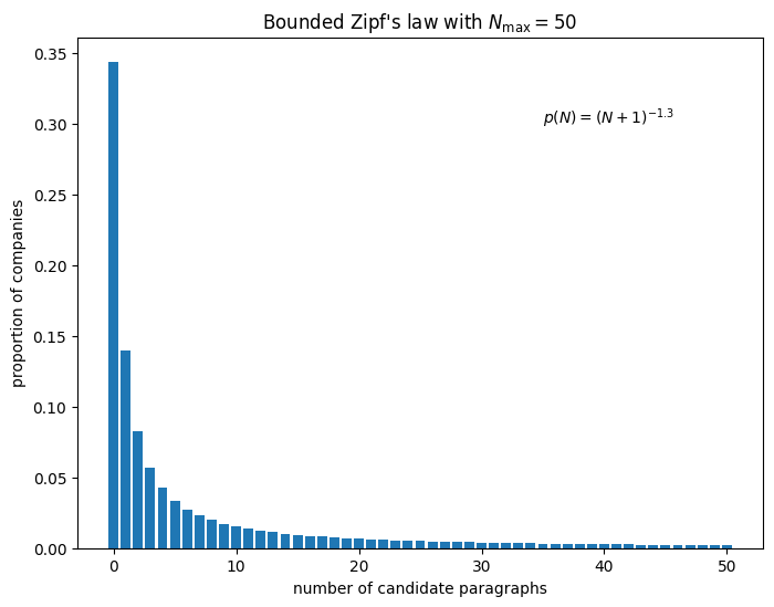
For a synthetic example, let’s say the distribution of the number of candidate paragraphs \(N\) follows a power-law, truncated to a max of 50 paragraphs because this roughly matches distributiones I’ve seen and the tail of the power law is too long for our purposes. Over a third of companies do not have any candidate paragraphs, while the remainder have one or more.
For each \(N\), the number of paragraphs tagged as positive \(K\) is a binomial random variable with some probability \(p\). To generate the synthetic dataset, we also need the confusion matrix which captures the ML model performance. Here’s an example for the case of a model evaluated on 250 data points:
| \(X = 1\) | \(X = 0\) | |
|---|---|---|
| \(\hat{X} = 1\) | TP = 135 | FP = 15 |
| \(\hat{X} = 0\) | FN = 30 | TN = 70 |
This is a decent model for our purposes, in that the precision is 0.9 and the recall is 0.82, giving \(F_1 = 0.86\). From this, we can compute the conditional propobabilities used in our equation:
\[P(X = 0 \vert \hat{X} = 1) = \frac{\text{FP}}{\text{TP} + \text{FP}} = 0.1\] \[P(X = 0 \vert \hat{X} = 0) = \frac{\text{TN}}{\text{TN} + \text{FN}} = 0.7\]Additionally, the ground truth probability \(p\) that any one paragraph is relevant (the prevalence) must be consistent with the confusion matrix:
\[p = \frac{\mathrm{TP} + \mathrm{FN}}{\mathrm{TP} + \mathrm{FP} + \mathrm{FN} + \mathrm{TN}} = 0.66\]With these numbers, we can generate a synthetic dataset for a universe of \(M = 1000\) companies. For the true label \(X\) of each paragraph, we introduce errors by flipping it with the following probabilities:
\[P(\hat{X} = 0 \vert X = 1) = \frac{\mathrm{FN}}{\mathrm{TP} + \mathrm{FN}}\] \[P(\hat{X} = 1 \vert X = 0) = \frac{\mathrm{FP}}{\mathrm{TN} + \mathrm{FP}}\]The resulting dataset is a set of 1000 rows, one for each company, specifying the number of candidate paragraphs \(N\) for that company, how many \(K\) are relevant, and how many \(K_\mathrm{pred}\) the model marked as relevant:
| \(N\) | \(K\) | \(K_\mathrm{pred}\) |
|---|---|---|
| 2 | 2 | 1 |
| 6 | 5 | 4 |
| 0 | 0 | 0 |
| 2 | 1 | 1 |
| 20 | 12 | 14 |
| … | … | … |
Now we can compute the fraction of companies which discuss a given topic, and apply our correction formula and check that the result is closer to the ground truth:
\[\begin{align} \mathrm{ground\,truth}&: \mathbb{E}(Y) = 608 / 1000 = 0.608 \\ \mathrm{predicted}&: \mathbb{E}(\hat{Y}) = 592 / 1000 = 0.592 \\ \mathrm{corrected}&: \mathbb{E}(Y) = 606 / 1000 = 0.606 \end{align}\]The corrected value is closer to the ground truth than the predicted value!
Discussion
I was surprised by the small magnitude of bias generated by model errors. In the above example, the bias was around 1.5%, which is a minor effect given my experience with systematic errors from other parts of the data generation and modeling pipeline. Playing around with the values in the confusion matrix, it appears that:
-
The bias increases as the difference between the precision and recall grows
-
The bias does not depend strongly on the prevalence of positives
There is a negative correlation when the bias is plotted against the difference between the precision and recall.
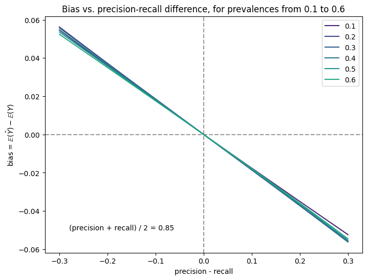
This makes sense: when the precision is higher than the recall, the model is missing more paragraphs than it is catching, leading to an under-report of the fraction of companies discussing a given topic, meaning the bias is negative. As the prevalence is swept from 0.1 to 0.6, the bias hardly changes. Finally, changing the overall performance of the model (in the above plot, we symmetrically varied the precision and recall about 0.85) does not strongly affect the bias either.
Finally, a note on correlations: this derivation is predicated on the fact that the labels for the paragraphs are independent Bernoulli variables. However, it’s possible that this is not true: for a given company, if one candidate paragraph discusses a given topic, say carbon emissions, it may be more likely that other candidates paragraphs for the same company will also discuss carbon emissions. These are correlated Bernoulli variables, and there is work on generating and fitting data to such models [1] [2]. I have yet to explore the direction and magnitude of the effect of correlations.
To summarize, in the uncorrelated case, we can correct for bias when aggregating per-paragraph tags to a company level, but this bias is only significant when the classifier is skewed towards either precision or recall.
Appendix: simulation code
import numpy as np
from scipy import stats

# for reproducibility
np.random.seed(3)

# construct bounded power law distribution
Nmax = 50
loc = -1
a = 1.3

x = np.arange(0, Nmax+1)
weights = (x - loc) ** (-a)
weights /= weights.sum()
bounded_zipf = stats.rv_discrete(name='bounded_zipf', values=(x, weights))

# number of companies
M = 1000

# number of paragraphs per company
N = bounded_zipf.rvs(size=M)

# quality of classifier (confusion matrix)
tp, fp, fn, tn = 135, 15, 30, 70

# number of relevant (positive) paragraphs per company
prevalence = (tp + fn) / (tp + fp + fn + tn)
print(f"prevalence (paragraph level) = {prevalence}")
K = stats.binom.rvs(N, prevalence)

# ground truth fraction of companies which discuss topic
EY = np.sum(K > 0)
print(f"{EY} / {M} = {EY / M:.2f} companies discuss the topic")

p01 = fp / (tp + fp)
p00 = tn / (fn + tn)
print(f"P(true = 0 | pred = 1) = {p01}, P(true = 0 | pred = 0) = {p00}")

print(f"precision = {tp / (tp + fp):.2f}, "
      f"recall = {tp / (tp + fn):.2f}, "
      f"F1 = {2*tp / (2*tp + fp + fn):.2f}")

# introduce errors based on classifier quality
Kpred = stats.binom.rvs(K, tp/(tp+fn)) + stats.binom.rvs(N-K, fp/(tn+fp))

# preview first 10 samples
print("    N =", N[:10])
print("    K =", K[:10])
print("Kpred =", Kpred[:10])

# ground truth and jittered expectations
print(f"E(Y) ground truth = {np.sum(K > 0)} / {M} = {np.sum(K > 0) / M:.6f}")
print(f"E(Y*) predicted   = {np.sum(Kpred > 0)} / {M} = {np.sum(Kpred > 0) / M:.6f}")

# corrected expectation value (should equal ground truth)
EYp = M - np.sum(p01**Kpred * p00**(N-Kpred))
print(f"E(Y) corrected    = {EYp:.0f} / {M} = {EYp / M:.6f}")

# Example output:
#
# prevalence (paragraph level) = 0.66
# 608 / 1000 = 0.61 companies discuss the topic
# P(true = 0 | pred = 1) = 0.1, P(true = 0 | pred = 0) = 0.7
# precision = 0.90, recall = 0.82, F1 = 0.86
#     N = [ 2  6  0  2 20 21  0  0  0  1]
#     K = [ 2  5  0  1 12 12  0  0  0  1]
# Kpred = [ 1  4  0  1 14  9  0  0  0  1]
# E(Y) ground truth = 608 / 1000 = 0.608000
# E(Y*) predicted   = 592 / 1000 = 0.592000
# E(Y) corrected    = 606 / 1000 = 0.606341