Let’s say someone hands you a coin that may or may not be unfair. How many times do you need to flip it to confidently determine whether it’s biased towards heads?

It’s a contrived question because I’ve never come across a biased coin in real life. Maybe it’s because I haven’t looked hard enough! Regardless, it’s an example of the more general problem of sample size determination as applied to Bernoulli trials.

I’ll use the coin flipping example in this post, but here are two realistic problems that are equivalent:

1. How many impressions do I need to serve to determine whether my new ad reaches a target conversion threshold of 2.5%?

2. How many positive test samples do I need to feed my classifier to confirm whether its recall is greater than 70%?

Inspired by Prof. Keith Goldfeld’s post (check it out, he’s got some useful literature references), we’re going to solve this using Bayesian inference, and do enough math to simplify the equations so that the can be computed on a laptop.

End-to-end simulation

The end result of this section will be an equation for the probability that we’re confident whether the coin is biased towards heads, and we’ll get there by reasoning through an end-to-end simulation.

Aside: what does the word “confident” mean in this context? See below!

A key input to the equation is the number of times \(N\) we choose to flip the coin. Intuitively, the equation should tell us that:

• the larger the number of coin flips, the higher the probability we can confidently proclaim the coin to be biased

• the smaller the actual bias of the coin, the lower the probability we’ll be able to detect whether the coin is unfair at a fixed number of clips

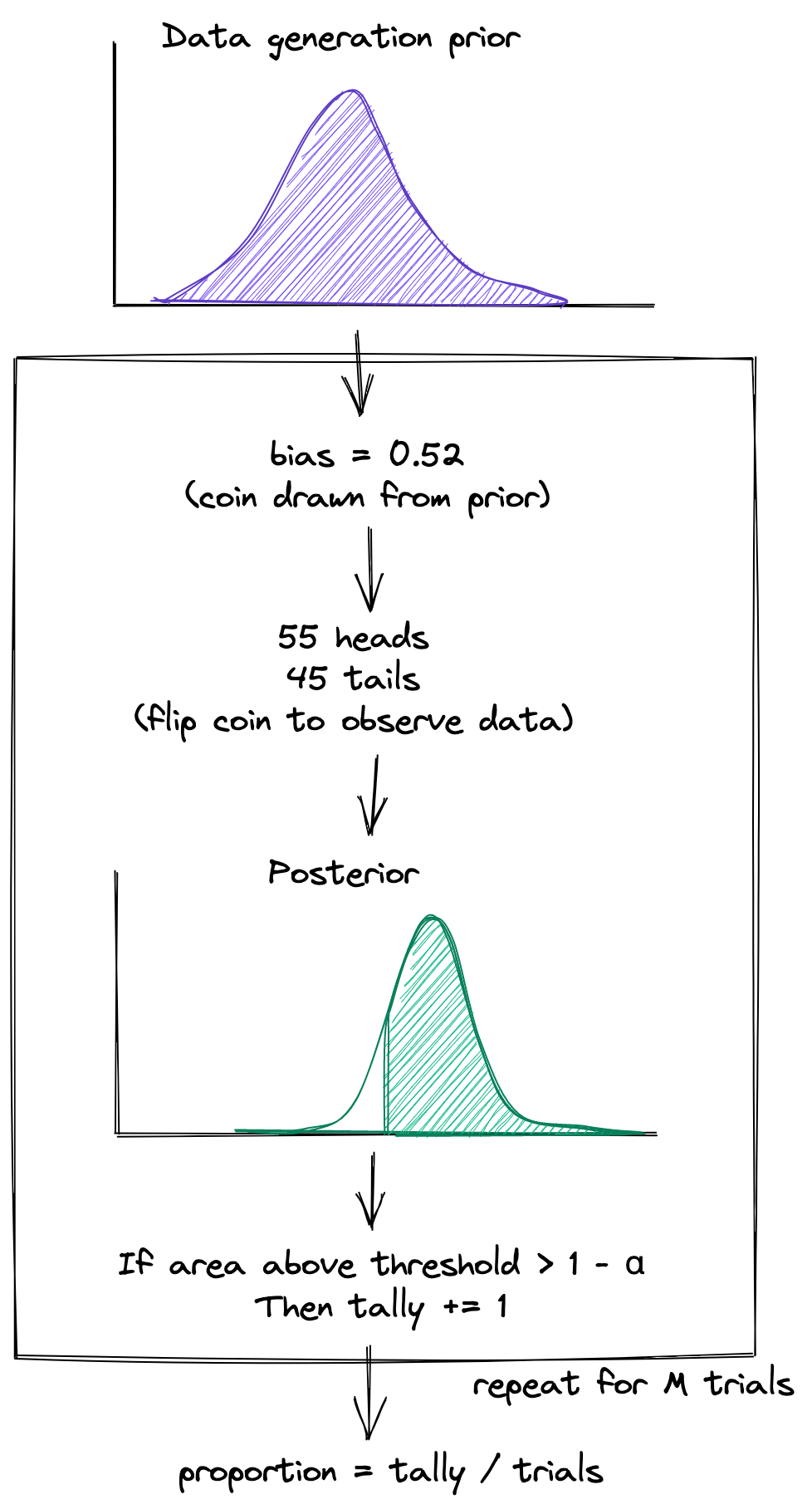
The steps of the simulation are as follows:

1. Since we don’t know a priori the bias of the coin, make a guess of its distribution by defining a data generation prior \(P_\mu(\theta_0)\) and sample a possible bias \(\theta_0\) from \(P_\mu\).

2. Flip the biased coin \(\theta_0\) a fixed number of times \(N\) to generate the data \(\mathcal{D}_N = (k, N-k)\), where \(k\) is the number of heads and \(N-k\) is the number of tails. In other words, sample \(\mathcal{D}_N\) from the likelihood \(P(\mathcal{D}_N \vert \theta_0)\).

3. Given the data \(\mathcal{D}_N\), compute the probability that the estimated bias \(\theta\) exceeds some threshold \(\theta_t\) by using the posterior \(P_\lambda(\theta > \theta_t \vert \mathcal{D}_N)\). For checking whether the coin is biased towards heads, set \(\theta_t = 0.5\). Note: an input to the posterior is a data analysis prior \(P_\lambda(\theta)\), which I’ll discuss below.

4. If the probability is greater than or equal to \(1 - \alpha\), which is our confidence level, add one to a running tally \(T\). Often, \(\alpha\) is set to \(0.05\), so that we are \(95\%\) confident.

5. Repeat steps 1-4 \(M\) times, and report the probability \(T/M = \beta\) at the end. The quantity \(\beta\) is the proportion of experiments which would result in a confident determination of the fairness of the coin.

To convert the simulation procedure into an equation, chain steps 3 and 4 together:

This is the boolean quantity that tallies whether we can confidently determine the biased-ness for a single experiment resulting in data \(\mathcal{D}_N\).

I want the proportion of all experiments that result in confident determination (steps 1, 2 and 5), which means taking the expected value over the distributions for \(\mathcal{D}_N\) and \(\theta_0\).

To notate mathematically, use the indicator function \(\mathbb{1}_A(\mathcal{D}_N)\) where:

to arrive at:

This is the equation we’ll implement. It looks complicated, but we’ll break down each factor in this post. I want to note a few things:

• Operationally, it’s a one-dimensional definite integral and a finite sum. This means we have a chance at numerically evaluating it.

• The right hand side is a function of three quantities: the number of data points \(N\), the threshold \(\theta_t\), a confidence level \(\alpha\). The left hand side is the proportion of successful experiments \(\beta\). If we input three of these four variables, our code should be able to solve for the fourth.

• There are two parameters \(\lambda\) and \(\mu\) characterizing the prior distributions.

In the next section, we’ll work out the equations explicitly for Bernoulli trials using conjugate priors.

Step by step

No, I’m not referring to the sitcom or the song by the New Kids on the Block.

1 - Data generation prior

This is a classic chicken-and-egg problem: the number of flips required depends on the magnitude of unknown bias \(\theta_0\), which we don’t know. So we make an educated guess for its distribution, codified in the data generation prior \(P_\mu(\theta_0)\).

We’ll use a beta distribution:

where \(\mu\) is shorthand for \(\mu_1\) and \(\mu_2\).

Let’s say we want to simulate a case where the coin is somewhat biased towards heads, so I choose \(\mu_1 = 6\) and \(\mu_2 = 4\).

2 - Likelihood

The likelihood is the probability of observing a certain number of heads and tails \(\mathcal{D}_N\), given the bias parameter \(\theta_0\). A coin flip is a Bernoulli trial. Repeated coin flips result in a Binomial distribution:

3 - Posterior

Time to apply Bayesian inference.

Step into the shoes of the experimenter: you’re handed a coin with an unknown bias \(\theta\) and observe \(k\) heads after \(N\) flips. Bayes theorem tells you how to update your beliefs:

But what do you choose as your prior \(P_\lambda(\theta)\)?

The point Wang and Gelfand [1] make is that the prior used to generate (or “sample”) the data Step 1 need not be the same prior used to analyze (or “fit”) the data in this step. This is the two-priors approach [2].

• When analyzing the data to fit the model, it is usually preferable to let the data drive the inference, so the analysis prior \(P_\lambda(\theta)\) is encouraged to be relatively uninformative.

• In contrast, the data generation prior encapsulates “what if” scenarios. We don’t want to design trials taking into consideration wildly improbable values of the bias, so it makes sense for \(P_\mu(\theta_0)\) to be less conservative and only have weight in a smaller, reasonable range of biases.

Back to the data analysis prior. I’ll again choose a beta prior because it is conjugate to the likelihood, which simplifies the math:

but I will set \(\lambda_1 = \lambda_2 = 1\), which specifies a uniform prior. Working through the math results in a posterior which is again a beta distribution:

What we want in this step is the probability the estimated bias \(\theta\) exceeds a some threshold \(\theta_t\). With the posterior in hand, integrate it:

The regularized beta function \(I_\theta\) is the CDF of the beta distribution.

4 - Confidence level

Checking whether the output probability in Step 3 is greater than \(1 - \alpha\) is equivalent to

This is a simple computation since most statistics libraries provide the CDF of the beta distribution.

5 - Expectation

Take the expected value of Step 4 over the probability distributions of Step 1 and 2:

Because we chose a beta prior for \(\theta_0\), its integral results in a beta-binomial distribution:

The final equation for the proportion of experiments resulting in confident determination of the fairness of the coin involves using the indicator function to select out which beta-binomial coefficients to keep:

where

This equation is simple to implement with standard statistical libraries.

Python implementation

Implementing the equations does not require tricks for numerical stabilization and a direct translation of the above two formulas into code works just fine:

import numpy as np
import scipy.stats as stats

def indicator(k, n, alpha, theta_t, lambda_):
    a = k + lambda_[0]
    b = n - k + lambda_[1]
    return stats.beta.cdf(theta_t, a, b) < alpha

def beta(n, theta_t, alpha, mu, lambda_):
    k = np.arange(n + 1)
    bb = stats.betabinom.pmf(k, n, mu[0], mu[1])
    ind = indicator(k, n, alpha, theta_t, lambda_)
    return np.sum(bb * ind)

# example usage

n, theta_t, alpha = 100, 0.7, 0.05
mu = 86, 16
lambda_ = 1, 1

beta(n, theta_t, alpha, mu, lambda_)  # 0.9025361931661403

The point is that it’s quite short, and only takes a few milliseconds to run on my old 2018 Macbook Air.

Sample size determination

With the requisite tools in hand, let’s turn to the business of determining sample sizes.

For the first example, suppose we want to know how many samples are needed to detect a coin with a large bias towards heads, say with \(\theta_0\) between \(0.6\) and \(0.9\). From fiddling with parameters, choosing \(\mu_1 = 10\) and \(\mu_2 = 3\) results in a data generation prior with significant weight where we desire:

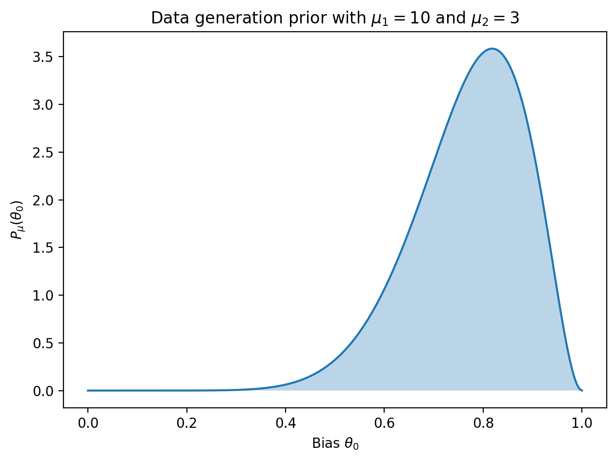
Now we can compute the proportion of posterior distributions meeting the 95% threshold as a function of the number of samples.

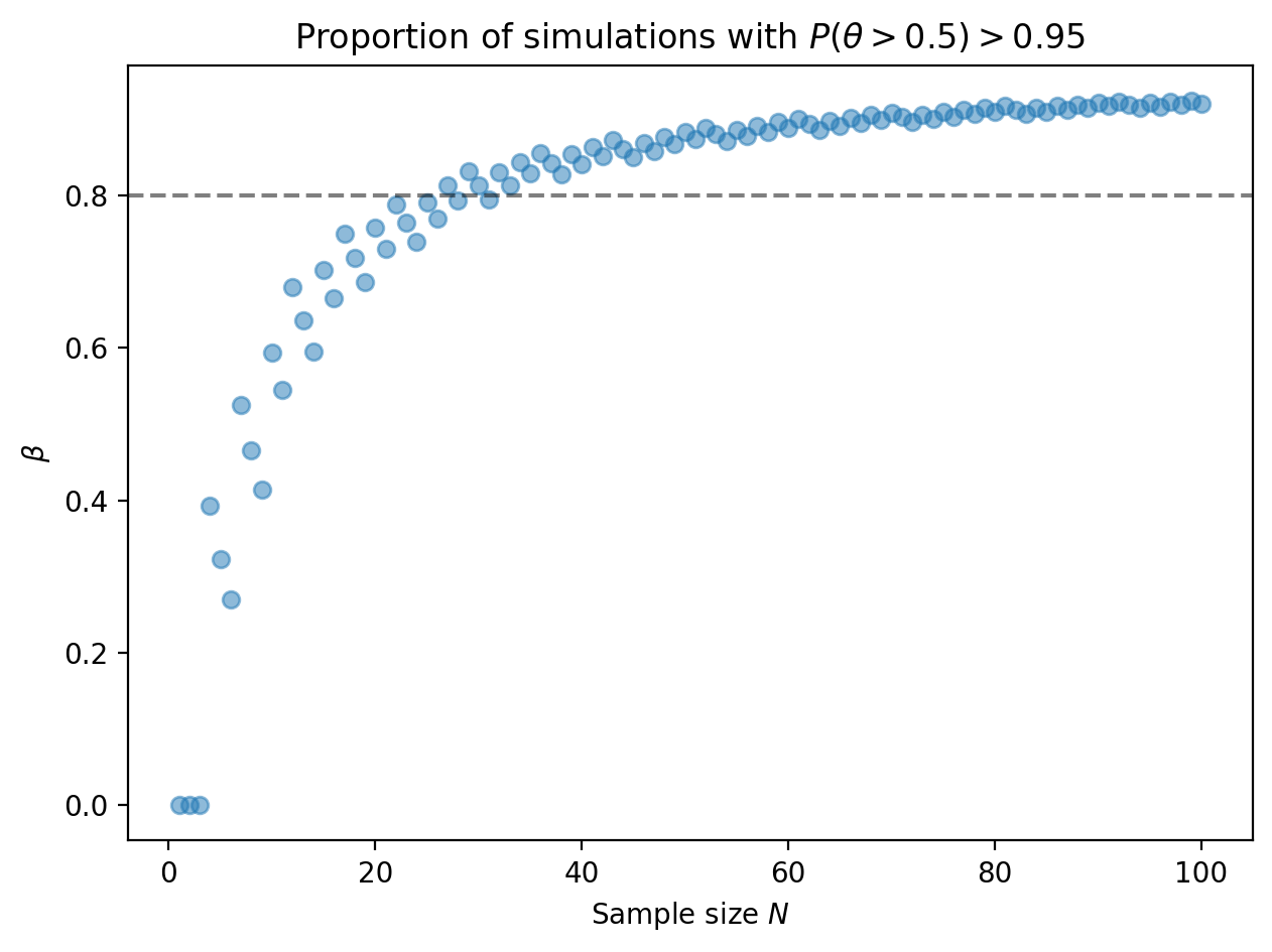
For a strongly biased coin, at around 30 samples, 80% of the posterior distributions will lead us to conclude that the coin is indeed biased.

Why does the proportion zig-zag? The reason is due to the discreteness of the number of posteriors passing the \(1 - \alpha\) threshold. (More discussion below.)

For the second example, suppose we want detect a coin with a very small bias, say 51-49 towards heads. Choosing \(\mu_1 = 51000\) and \(\mu_2 = 49000\) results in a data prior with a sharp peak at \(\theta_0 = 0.51\):

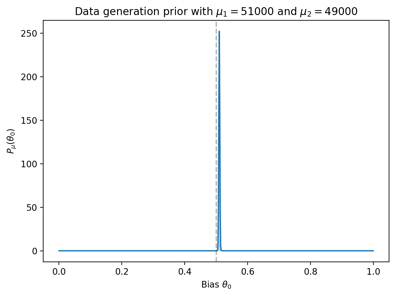
For such a small bias, we expect to require a large number of samples:

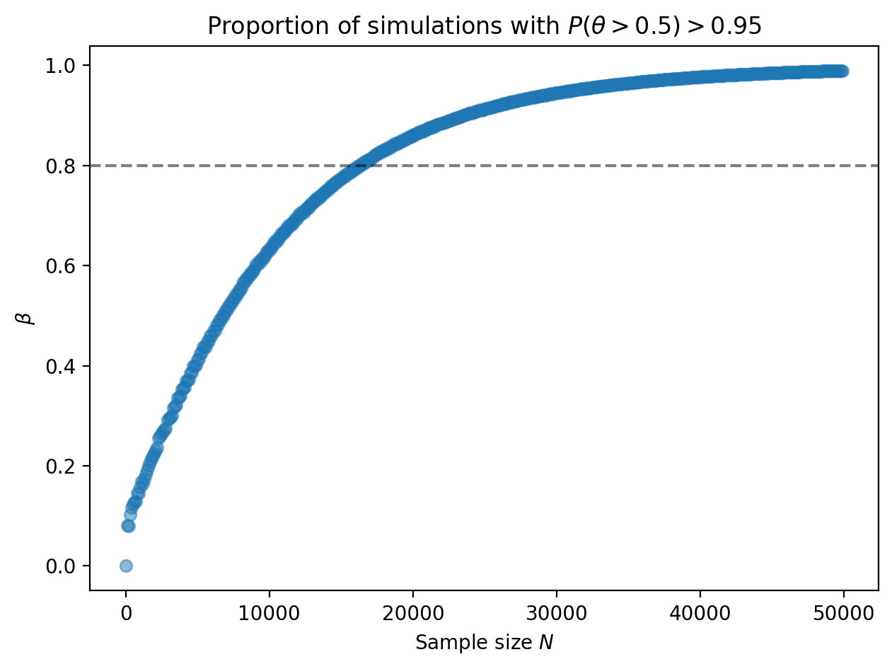
Conclusion: for a 1% bias, over 16000 samples are required so that 80% of the posterior distributions will lead us to conclude that the coin is biased towards heads.

A useful trick for solving for the sample size given the other three parameters is to use the bisect module from the Python Standard Library and write a lightweight class which provides a list-like interface into the beta() function:

from bisect import bisect

def sample_size(threshold, theta_t, alpha, mu, lambda_):
    class C:
        def __getitem__(self, n):
            return beta(n, theta_t, alpha, mu, lambda_)
    n = 1
    while beta(n, theta_t, alpha, mu, lambda_) < threshold:
        n *= 2
    c = C()
    return bisect(c, threshold, hi=n)

sample_size(0.8, 0.5, 0.05, (51000, 49000), (1,1))  # 16230

Effects of discreteness

Why does the proportion of trials which can confidently detect bias exhibit zig zags? Zooming in to the plot of proportion vs. sample size, we see jumps at \(N = 4, 7, 10\).

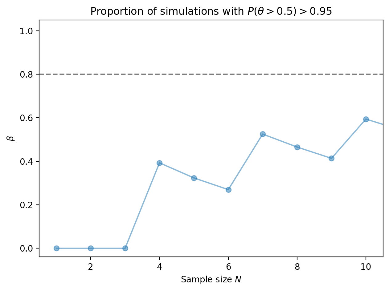
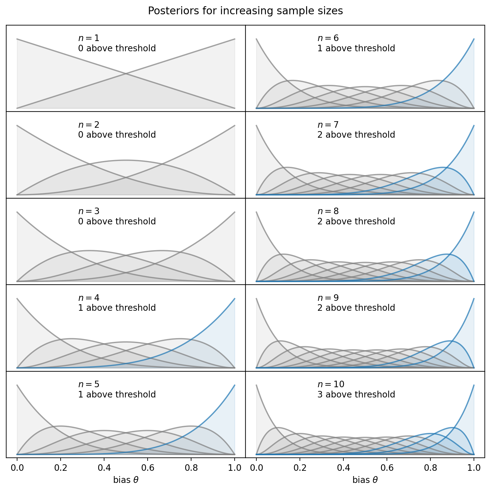
Take a look at the posteriors: for a given sample size \(N\), there are \(N+1\) posteriors corresponding to observing \(0, 1, 2, \ldots, N\) heads. The number of those posteriors with over 95% density above the threshold \(\theta = 0.5\) increments at somewhat arbitrary values of the sample size.

No posteriors pass the threshold for \(N = 1, 2, 3\). But at \(N = 4\), one of the posteriors has over 95% density above \(\theta = 0.5\) (colored in blue below), corresponding to a jump in the proportion of successful trials. The same pattern holds for sample sizes of 7 and 10, where additional posteriors pass the threshold.

Does this behavior make sense? I frankly am uncertain, but perhaps others have encountered the same issue even if I am unaware.

Summary

While Bayesian approaches usually require Monte Carlo simulations due to the intractibility of the formulas to analytic methods, the case of Bernoulli trials is amenable to analytic manipulation. It’s also worth doing because a few commonly use metrics–namely accuracy, precision and recall–can be reduced to the framework of Bernoulli trials.

Sample size determination may appear to be a rigorous discipline given the amount of mathematics required, especially in the Bayesian approach, but in practice the prior assumptions aren’t known with much accuracy. Returning to the example of “how many positive test samples do I need to feed my classifier to confirm whether its recall is greater than 70%” posed in the introduction:

• The biggest uncertainty is the parameters of the data generation prior. We cannot be more precise about the computed sample size than the amount of certainty we have over what we think is the model’s recall.

• How high a proportion do we want to succeed? Is 80% high enough?

• How exact is the 70% requirement? If the threshold comes from product or business constraints, sometimes it’s not rigid, especially if it’s in the context of non-critical user products (for example, the difference between 70% and 75% recall for search over news articles may be a non-issue for clients, while the difference between 95% and 99% recall for identification of pedestrians is critical for autonomous vehicles).

In practice, it makes sense to jitter the numbers to create a table of possible scenarios and make a decision on the sample size based on a combination of statistical power and other factors like annotation cost and business timelines.